Anti-aliasing Polygon Edges for Scanline Rendering
Anti-aliasing is something many of us take for granted these days. Certainly in the realtime world there are a number of well-known techniques using clever manipulation of graphics hardware (MSAA, FXAA, TXAA) each with variations in quality (2x, 4x, 8x, 16x) with associated higher GPU processing costs. But outside of the realtime world, there are still cases where we may have to implement a high-quality anti-aliasing solution.
Recently, for example, I was working on a rotoscoping plugin for Nuke. Rotoscoping tools render polygons that are used as masks in compositing. Most compositing tools use a traditional scanline-based approach to rendering, so my first step was to implement a polygon fill algorithm. This is a fast algorithm that works well but leaves jagged edges, and the end result cries out for anti-aliasing.
Approaches to Anti-Aliasing
Many papers have been written about anti-aliasing over the years, with various approaches along the way. Ed Catmull's 1978 paper was an early attempt to answer the question "how much of this pixel is covered by this polygon?". His analytical approach was relatively expensive and in 1984 Loren Carpenter came up with a much faster alternative called the A-Buffer. There have been quite a few variations on this approach over the years.
It's also possible to use approaches at a much higher level. In ray tracing it's common to use scene-wide anti-aliasing approaches such as super-sampling, adaptive sampling, or stochastic sampling. These approaches yield high quality results, but can be quite expensive.
A Review of the A-Buffer Algorithm for Coverage Estimation
I had certain specific requirements for my roto scanline renderer:
- I only need a single channel output (alpha channel) and I can assume each poly has identical attributes
- polygons can have an arbitrary number of edges/vertices
- polygons should still be able to render correctly even if they self-intersect ("bow tie polygons")
- the algorithm shouldn't be substantially slower than the non-anti-aliased version. i.e. I only want to spend the extra processing on pixels that need it.
I decided on a variation of the A-Buffer algorithm for coverage estimation. An A-Buffer does anti-aliasing by sampling the area of polygons in a pixel using a 4x8 sub-pixel grid. The algorithm begins as follows:
- for each scanline row, calculate which polygons intersect that row
- for each pixel in the row, calculate which polygons intersect that pixel
- clip those polygons to the pixel
At this point you have a set of edges that intersect the pixel.
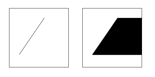
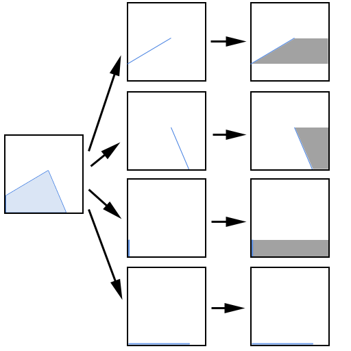
Before we jump into the A-Buffer bitmask technique, let's step back and look at this analytically. The first thing to understand is that it's possible to take those edges and reproduce the original polygon within the pixel using an interesting technique: For each edge, you can draw out a trapezoid by pushing that edge to the right until it passes over the rightmost edge of the pixel.

Do this for each edge that intersects the cell:

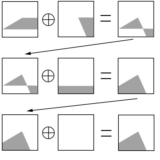
Then XOR the results together:

What you're left with is drawn areas where the polygon is in the cell and non-drawn areas where it isn't in the cell.
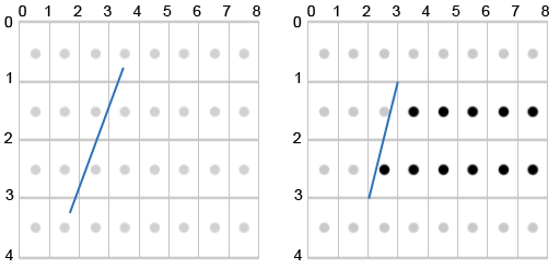
This key idea is the cornerstone of the A-Buffer algorithm, but it still doesn't give us any useful coverage information. We've just reproduced the original polygon using it's edges. We want coverage. It's here that the A-Buffer gets really clever. It uses a 4x8 grid underlying the pixel to quickly calculate an approximation of the coverage percentage of the polygon in the pixel.

But you don't need to do the math for each edge for every pixel. All possible combinations can be pre-computed and placed in a lookup table. The quantization of the edge to grid intersections reduces the total number of possible combinations of x1,y1,x2,y2 to 5 x 5 x 9 x 9 = 2025 combinations. At 4 bytes (32 bits) per lookup entry, that's a total of 8k for a lookup table which you can precompute.
Once you have the mask for the edge, you can use bitwise XOR to accomplish the same geometric XOR operation as in our earlier analysis.
So, once you've clipped the polygon edges to the pixel, the final algorithm looks like:
- Start with an empty mask:
uint32_t mask = 0; - For each edge: Quantize and scale X to 0-8, Y to 0-4 for the start and end points Lookup into your table using those quantized integer values:
uint32_t edgemask = maskTable[x1][y1][x2][y2];XOR that maskmask = mask ^ edgemask; - Once all edges have been processed, find the number of bits remaining in the mask and divide by 32 to get an aproximate percent coverage of the pixel. You can certainly iterate through each bit and count them, or use more clever techniques, but most modern processors have a single instruction which can do the work for you:
#include "intrinsics.h" #pragma intrinsic(__popcnt32) ... int numBits = (int) __popcnt32(mask);
Though if you're shipping a commercial product, I encourage you to go to the trouble of determinining whether that instruction exists on the CPU that you're running on before executing it, and use an alternative technique otherwise. Using that call on a machine that doesn't support popcnt has undefined results.
You can then use this percent coverage as an opacity value to blend the polygon into the image. The original A-Buffer paper goes into detail regarding how to do this blending correctly, even when fragments intersect in Z, but I won't cover that here, since my primary concern is coverage estimation.
Implementation and Optimization
An obvious modern improvement to the A-Buffer coverage estimation is to increase the grid size from 4 x 8 to 8 x 8. This doubles the number of sample points and allows X and Y to be equal partners in the coverage algorithm. This is now possible because all modern desktop CPUs use 64 bit registers internally and there's no added processing cost to XOR two 64 bit values together vs two 32 bit values. The modifications to the 4 x 8 algorithm are simple:
- Precompute a larger grid. It will now requires 9 x 9 x 9 x 9 entries of 64 bit values. This is quite a bit larger: 9 x 9 x 9 x 9 = 6561 entries. Each entry is now 8 bytes, so the total size is now 52k. That may have been excessive for a machine in 1984, but it's quite reasonable for a modern PC and is still small enough to play nicely with L1 and L2 cache. (That said, the 52k size will certainly cause more L1 cache misses than 8k, so there may be some minor performance trade-off here.)
- When looking up into the table, quantize and scale X to 0-8 and Y to 0-8 for the start and end points.
- Use the 64 bit version of popcnt:
return (int) __popcnt64(mask);
Next up is the consideration of clipping polygon edges to the scanline and pixel. When it comes to pruning polygon edges, it pays to be as aggressive as possible as early as possible. If you have a bounding box for your polygon, use it to prune it out from scanline processing on rows that it doesn't cover. For each polygon that crosses the scanline, clip that polygon to the scanline. Note that it's important that you clip the polygon to the scanline. You can't just extract the edges that cross the scanline. Even though those edges on the top and bottom won't generate usable masks themselves (they'll always generate blank masks), they're important because when clipping to the pixel, they'll end up generating edges along the left edge of the pixel, which are vitally important as they do create important mask information.
I used a modified Sutherland-Hodgman algorithm. Specifically, since I knew I was only going to ever clip along pixel edges, I created two functions for clipping: one to clip along vertical lines (with a parameter that controlled left/right) and another for horizontal lines (with a parameter that controlled up/down).
Here's some sample code based upon Sutherland-Hodgman simplified for clipping along a horizontal line:
	void clipToHorizontalLine(float y, float norm,
			const std::vector<Vector2>& ptsIn,
			std::vector<Vector2>& ptsOut)
	{
		ptsOut.clear();
		int nPoints = (int) ptsIn.size();
		int nodes = 0;
		int j = nPoints - 1;	// i is the current vertex, j is the previous
		for (int i = 0; i < nPoints; i++)
		{
			Vector2 current = ptsIn[i];
			Vector2 previous = ptsIn[j];
			// If current is on the correct side
			if ((current.y - y) * norm <= 0)
			{
				// If previous is NOT on correct side
				if ((previous.y - y) * norm > 0)
				{
					// Calculate the intercept
					float px1 = (current.x + (previous.x - current.x)
						      * (y - current.y) / (previous.y - current.y));

					// Push the intersect. Don't push the other one,
					// because it's not on the correct side.
					ptsOut.push_back(Vector2(px1, y));
				}

				// Push the current, because it's on the correct side
				ptsOut.push_back(current);
			}
			// If previous is on the correct side
			else if ((previous.y - y) * norm <= 0)
			{
				// Calculate the intercept
				float px1 = (current.x + (previous.x - current.x)
						  * (y - current.y) / (previous.y - current.y));

				// Push the intersect
				ptsOut.push_back(Vector2(px1, y));
			}
			j = i;
		}
	}
Clipping along a vertical line is similar with X and Y swapped in appropriate places.
The A-Buffer coverage algorithm is certainly a performance win over doing a full analytical coverage calculation for a pixel, but it's still not fast enough by itself for filling large polygons that cover hundreds of thousands of pixels or more. There is a way, though, to skip the clipping and coverage calculation for most pixels. Any pixel that is entirely inside or entirely outside a polygon can have a much simpler algorithm applied to it. To do this, once I have the edge list for the scan line, I also generate a boolean array for the scanline which I call the "complex" table. The idea of the "complex" table is that if it's set to TRUE for a pixel, then I need to perform full A-Buffer calculations for the pixel, otherwise, I can use the simpler technique.
To calculate the "complex" table, I simply iterate through the edge list I've generated for the scanline and look for edges where the Y values aren't the same between the start and end points of the edge. It's only these sorts of edges that cause a change in the mask from one pixel to the next.
When I detect these sorts of edges, I fill in the "complex" table with TRUEs from the beginning X of the edge to the end X, being careful to not go outside the bounds of the table:
	void setComplex(const std::vector<Vector2>& pts, std::vector<char>& complex)
	{
		int r = (int)complex.size();
		int nPoints = (int) pts.size();
		int j = nPoints - 1;
		for (int i = 0; i < nPoints; i++)
		{
			if (pts[i].y != pts[j].y)
			{
				int ix1 = (int) floor(pts[i].x);
				int ix2 = (int) floor(pts[j].x);
				if (ix1 > ix2)
					std::swap(ix1, ix2);

				if (ix1 < r && ix2 >= 0) {	 // Are any pixels affected?

					if (ix2 >= r)	// Clamp to the complex table
						ix2 = r - 1;
					if (ix1 < 0)	// Clamp to the complex table
						ix1 = 0;

					for (int x = ix1; x <= ix2; ++x)
						complex[x] = 1;
				}
			}
			j = i;
		}
	}
Once I have this table, I can iterate through the pixels in the scanline and only perform clipping and coverage tests when I have to. I always perform the full clipping and coverage when it's complex, but if it's "simple", then I only perform it for the first simple pixel after the last complex pixel, and then copy the results for each subsequent simple pixel until I hit the next complex pixel. It sounds more complicated than the actual code. Here I'm generating an alpha channel for my rotoscoping tool, adding the calculated coverage to whatever's already in the "data" buffer. I've merged all the roto polys into one giant edge list so that they perform XOR calculations with each other (so you can easily generate "holes" by having polys inside of other polys).
	bool calculateCoverage = true;
	float currentCoverage = 0.0f;

	// Calculate scanline between x and r
	for (int px = x; px < r; ++px)
	{
		bool isComplex = complex[px];
		// If the current cell is complex, we need to calculate it.
		calculateCoverage |= isComplex;

		if (calculateCoverage)
		{
			// Calculate the A-Buffer coverage for this cell.
			std::vector<Vector2> pts1;
			std::vector<Vector2> pts2;
			// Clip edges to the pixel
			clipToVerticalLine((float) px,        -1.0f, edges, pts1);
			clipToVerticalLine((float) px + 1.0f, +1.0f, pts1, pts2);
			currentCoverage = applyABuffer((float)px, (float)y, pts2);
			// Our coverage can be used in the next pixel
			// only if this pixel is simple
			calculateCoverage = isComplex;
		}

		// Apply the coverage to the pixel
		// Only do this logic if there's something to apply
		if (currentCoverage != 0) {
			float val = data[px];
			val += currentCoverage;
			if (val > 1.0f)
				val = 1.0f;
			data[px] = val;
		}
	}
Real scanline rendering of a scene where each poly has different attributes is more complicated, of course. You need to think about fragments and how to blend together fragments in a pixel. Loren Carpenter's original A-Buffer paper has an excellent discussion of this.
Conclusion
The above algorithm generates nicely anti-aliased edges and only performs those anti-aliasing calculations on pixels which actually need anti-aliasing applied to them. It only touches each pixel once, and adds little overhead for pixels where no anti-aliasing is required. If you need to implement some sort of anti-aliasing, then hopefully this will have given you a bit of a head start.